Week 8 Notebook: Extending the Model
This week, we will look at graph neural networks using the PyTorch Geometric library: https://pytorch-geometric.readthedocs.io/. See [21] for more details.
import torch
import torch_geometric
device = torch.device("cuda:0" if torch.cuda.is_available() else "cpu")
from tqdm.notebook import tqdm
import numpy as np
local = False
import yaml

with open('definitions.yml') as file:
    # The FullLoader parameter handles the conversion from YAML
    # scalar values to Python the dictionary format
    definitions = yaml.load(file, Loader=yaml.FullLoader)

features = definitions['features']
spectators = definitions['spectators']
labels = definitions['labels']

nfeatures = definitions['nfeatures']
nspectators = definitions['nspectators']
nlabels = definitions['nlabels']
ntracks = definitions['ntracks']
Graph datasets
Here we have to define the graph dataset. We do this in a separate class following this example: https://pytorch-geometric.readthedocs.io/en/latest/notes/create_dataset.html#creating-larger-datasets
Formally, a graph is represented by a triplet \(\mathcal G = (\mathbf{u}, V, E)\), consisting of a graph-level, or global, feature vector \(\mathbf{u}\), a set of \(N^v\) nodes \(V\), and a set of \(N^e\) edges \(E\). The nodes are given by \(V = \{\mathbf{v}_i\}_{i=1:N^v}\), where \(\mathbf{v}_i\) represents the \(i\)th node’s attributes. The edges connect pairs of nodes and are given by \(E = \{\left(\mathbf{e}_k, r_k, s_k\right)\}_{k=1:N^e}\), where \(\mathbf{e}_k\) represents the \(k\)th edge’s attributes, and \(r_k\) and \(s_k\) are the indices of the “receiver” and “sender” nodes, respectively, connected by the \(k\)th edge (from the sender node to the receiver node). The receiver and sender index vectors are an alternative way of encoding the directed adjacency matrix.

from GraphDataset import GraphDataset
if local:
    file_names = ['/teams/DSC180A_FA20_A00/b06particlephysics/train/ntuple_merged_10.root']
    file_names_test = ['/teams/DSC180A_FA20_A00/b06particlephysics/test/ntuple_merged_0.root']
else:
    file_names = ['root://eospublic.cern.ch//eos/opendata/cms/datascience/HiggsToBBNtupleProducerTool/HiggsToBBNTuple_HiggsToBB_QCD_RunII_13TeV_MC/train/ntuple_merged_10.root']
    file_names_test = ['root://eospublic.cern.ch//eos/opendata/cms/datascience/HiggsToBBNtupleProducerTool/HiggsToBBNTuple_HiggsToBB_QCD_RunII_13TeV_MC/test/ntuple_merged_0.root']

graph_dataset = GraphDataset('gdata_train', features, labels, spectators, n_events=1000, n_events_merge=1,
                             file_names=file_names)

test_dataset = GraphDataset('gdata_test', features, labels, spectators, n_events=2000, n_events_merge=1,
                             file_names=file_names_test)
Processing...
Done!
Processing...
Done!
Graph neural network
Here, we recapitulate the “graph network” (GN) formalism [22], which generalizes various GNNs and other similar methods. GNs are graph-to-graph mappings, whose output graphs have the same node and edge structure as the input. Formally, a GN block contains three “update” functions, \(\phi\), and three “aggregation” functions, \(\rho\). The stages of processing in a single GN block are:
\( \begin{align} \mathbf{e}'_k &= \phi^e\left(\mathbf{e}_k, \mathbf{v}_{r_k}, \mathbf{v}_{s_k}, \mathbf{u} \right) & \mathbf{\bar{e}}'_i &= \rho^{e \rightarrow v}\left(E'_i\right) & \text{(Edge block),}\\ \mathbf{v}'_i &= \phi^v\left(\mathbf{\bar{e}}'_i, \mathbf{v}_i, \mathbf{u}\right) & \mathbf{\bar{e}}' &= \rho^{e \rightarrow u}\left(E'\right) & \text{(Node block),}\\ \mathbf{u}' &= \phi^u\left(\mathbf{\bar{e}}', \mathbf{\bar{v}}', \mathbf{u}\right) & \mathbf{\bar{v}}' &= \rho^{v \rightarrow u}\left(V'\right) &\text{(Global block).} \label{eq:gn-functions} \end{align} \)
where \(E'_i = \left\{\left(\mathbf{e}'_k, r_k, s_k \right)\right\}_{r_k=i,\; k=1:N^e}\) contains the updated edge features for edges whose receiver node is the \(i\)th node, \(E' = \bigcup_i E_i' = \left\{\left(\mathbf{e}'_k, r_k, s_k \right)\right\}_{k=1:N^e}\) is the set of updated edges, and \(V'=\left\{\mathbf{v}'_i\right\}_{i=1:N^v}\) is the set of updated nodes.

We will define an interaction network model similar to Ref. [1], but just modeling the particle-particle interactions. It will take as input all of the tracks (with 48 features) without truncating or zero-padding. Another modification is the use of batch normalization [23] layers to improve the stability of the training.
import torch.nn as nn
import torch.nn.functional as F
import torch_geometric.transforms as T
from torch_geometric.nn import EdgeConv, global_mean_pool
from torch.nn import Sequential as Seq, Linear as Lin, ReLU, BatchNorm1d
from torch_scatter import scatter_mean
from torch_geometric.nn import MetaLayer

inputs = 48
hidden = 128
outputs = 2

class EdgeBlock(torch.nn.Module):
    def __init__(self):
        super(EdgeBlock, self).__init__()
        self.edge_mlp = Seq(Lin(inputs*2, hidden),
                            BatchNorm1d(hidden),
                            ReLU(),
                            Lin(hidden, hidden))

    def forward(self, src, dest, edge_attr, u, batch):
        out = torch.cat([src, dest], 1)
        return self.edge_mlp(out)

class NodeBlock(torch.nn.Module):
    def __init__(self):
        super(NodeBlock, self).__init__()
        self.node_mlp_1 = Seq(Lin(inputs+hidden, hidden),
                              BatchNorm1d(hidden),
                              ReLU(),
                              Lin(hidden, hidden))
        self.node_mlp_2 = Seq(Lin(inputs+hidden, hidden),
                              BatchNorm1d(hidden),
                              ReLU(),
                              Lin(hidden, hidden))

    def forward(self, x, edge_index, edge_attr, u, batch):
        row, col = edge_index
        out = torch.cat([x[row], edge_attr], dim=1)
        out = self.node_mlp_1(out)
        out = scatter_mean(out, col, dim=0, dim_size=x.size(0))
        out = torch.cat([x, out], dim=1)
        return self.node_mlp_2(out)


class GlobalBlock(torch.nn.Module):
    def __init__(self):
        super(GlobalBlock, self).__init__()
        self.global_mlp = Seq(Lin(hidden, hidden),
                              BatchNorm1d(hidden),
                              ReLU(),
                              Lin(hidden, outputs))

    def forward(self, x, edge_index, edge_attr, u, batch):
        out = scatter_mean(x, batch, dim=0)
        return self.global_mlp(out)


class InteractionNetwork(torch.nn.Module):
    def __init__(self):
        super(InteractionNetwork, self).__init__()
        self.interactionnetwork = MetaLayer(EdgeBlock(), NodeBlock(), GlobalBlock())
        self.bn = BatchNorm1d(inputs)

    def forward(self, x, edge_index, batch):

        x = self.bn(x)
        x, edge_attr, u = self.interactionnetwork(x, edge_index, None, None, batch)
        return u

model = InteractionNetwork().to(device)
optimizer = torch.optim.Adam(model.parameters(), lr = 1e-2)
Define training loop
@torch.no_grad()
def test(model, loader, total, batch_size, leave=False):
    model.eval()

    xentropy = nn.CrossEntropyLoss(reduction='mean')

    sum_loss = 0.
    t = tqdm(enumerate(loader), total=total/batch_size, leave=leave)
    for i, data in t:
        data = data.to(device)
        y = torch.argmax(data.y, dim=1)
        batch_output = model(data.x, data.edge_index, data.batch)
        batch_loss_item = xentropy(batch_output, y).item()
        sum_loss += batch_loss_item
        t.set_description("loss = %.5f" % (batch_loss_item))
        t.refresh() # to show immediately the update

    return sum_loss/(i+1)

def train(model, optimizer, loader, total, batch_size, leave=False):
    model.train()

    xentropy = nn.CrossEntropyLoss(reduction='mean')

    sum_loss = 0.
    t = tqdm(enumerate(loader), total=total/batch_size, leave=leave)
    for i, data in t:
        data = data.to(device)
        y = torch.argmax(data.y, dim=1)
        optimizer.zero_grad()
        batch_output = model(data.x, data.edge_index, data.batch)
        batch_loss = xentropy(batch_output, y)
        batch_loss.backward()
        batch_loss_item = batch_loss.item()
        t.set_description("loss = %.5f" % batch_loss_item)
        t.refresh() # to show immediately the update
        sum_loss += batch_loss_item
        optimizer.step()

    return sum_loss/(i+1)
Define training, validation, testing data generators
from torch_geometric.data import Data, DataListLoader, Batch
from torch.utils.data import random_split

def collate(items):
    l = sum(items, [])
    return Batch.from_data_list(l)

torch.manual_seed(0)
valid_frac = 0.20
full_length = len(graph_dataset)
valid_num = int(valid_frac*full_length)
batch_size = 32

train_dataset, valid_dataset = random_split(graph_dataset, [full_length-valid_num,valid_num])

train_loader = DataListLoader(train_dataset, batch_size=batch_size, pin_memory=True, shuffle=True)
train_loader.collate_fn = collate
valid_loader = DataListLoader(valid_dataset, batch_size=batch_size, pin_memory=True, shuffle=False)
valid_loader.collate_fn = collate
test_loader = DataListLoader(test_dataset, batch_size=batch_size, pin_memory=True, shuffle=False)
test_loader.collate_fn = collate


train_samples = len(train_dataset)
valid_samples = len(valid_dataset)
test_samples = len(test_dataset)
print(full_length)
print(train_samples)
print(valid_samples)
print(test_samples)
920
736
184
1889
/usr/share/miniconda/envs/ml-latest/lib/python3.9/site-packages/torch_geometric/deprecation.py:13: UserWarning: 'data.DataListLoader' is deprecated, use 'loader.DataListLoader' instead
  warnings.warn(out)
Train
import os.path as osp

n_epochs = 10
stale_epochs = 0
best_valid_loss = 99999
patience = 5
t = tqdm(range(0, n_epochs))

for epoch in t:
    loss = train(model, optimizer, train_loader, train_samples, batch_size, leave=bool(epoch==n_epochs-1))
    valid_loss = test(model, valid_loader, valid_samples, batch_size, leave=bool(epoch==n_epochs-1))
    print('Epoch: {:02d}, Training Loss:   {:.4f}'.format(epoch, loss))
    print('           Validation Loss: {:.4f}'.format(valid_loss))

    if valid_loss < best_valid_loss:
        best_valid_loss = valid_loss
        modpath = osp.join('interactionnetwork_best.pth')
        print('New best model saved to:',modpath)
        torch.save(model.state_dict(),modpath)
        stale_epochs = 0
    else:
        print('Stale epoch')
        stale_epochs += 1
    if stale_epochs >= patience:
        print('Early stopping after %i stale epochs'%patience)
        break
Epoch: 00, Training Loss:   0.3590
           Validation Loss: 0.4111
New best model saved to: interactionnetwork_best.pth
Epoch: 01, Training Loss:   0.1760
           Validation Loss: 0.3918
New best model saved to: interactionnetwork_best.pth
Epoch: 02, Training Loss:   0.1709
           Validation Loss: 0.2485
New best model saved to: interactionnetwork_best.pth
Epoch: 03, Training Loss:   0.1742
           Validation Loss: 0.2379
New best model saved to: interactionnetwork_best.pth
Epoch: 04, Training Loss:   0.1491
           Validation Loss: 0.2254
New best model saved to: interactionnetwork_best.pth
Epoch: 05, Training Loss:   0.1261
           Validation Loss: 0.2602
Stale epoch
Epoch: 06, Training Loss:   0.1282
           Validation Loss: 0.3065
Stale epoch
Epoch: 07, Training Loss:   0.1186
           Validation Loss: 0.2528
Stale epoch
Epoch: 08, Training Loss:   0.1406
           Validation Loss: 0.2769
Stale epoch
Epoch: 09, Training Loss:   0.1058
           Validation Loss: 0.2603
Stale epoch
Early stopping after 5 stale epochs
Evaluate on testing data
model.eval()
t = tqdm(enumerate(test_loader),total=test_samples/batch_size)
y_test = []
y_predict = []
for i,data in t:
    data = data.to(device)
    batch_output = model(data.x, data.edge_index, data.batch)
    y_predict.append(batch_output.detach().cpu().numpy())
    y_test.append(data.y.cpu().numpy())
y_test = np.concatenate(y_test)
y_predict = np.concatenate(y_predict)
from sklearn.metrics import roc_curve, auc
import matplotlib.pyplot as plt
import mplhep as hep
plt.style.use(hep.style.ROOT)
# create ROC curves
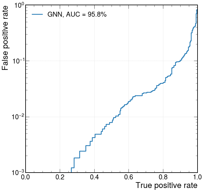
fpr_gnn, tpr_gnn, threshold_gnn = roc_curve(y_test[:,1], y_predict[:,1])
# plot ROC curves
plt.figure()
plt.plot(tpr_gnn, fpr_gnn, lw=2.5, label="GNN, AUC = {:.1f}%".format(auc(fpr_gnn,tpr_gnn)*100))
plt.xlabel(r'True positive rate')
plt.ylabel(r'False positive rate')
plt.semilogy()
plt.ylim(0.001, 1)
plt.xlim(0, 1)
plt.grid(True)
plt.legend(loc='upper left')
plt.show()