Lab 2: Numba#
Links:
https://carpentries-incubator.github.io/lesson-gpu-programming/02-cupy/index.html
https://docs.google.com/presentation/d/13MmOKh30IbRJo5sZ8ZujQFr1J3rhqDjA-0Qkfg7JZmE/edit#slide=id.p
https://indico.cern.ch/event/1019958/timetable/#43-cuda-and-python-with-numba
https://jakevdp.github.io/blog/2012/08/18/matplotlib-animation-tutorial/
Simple stuff#
Even if you’ve used Numba before, let’s start with the basics.
In fact, let’s start with NumPy itself.
NumPy#
import numpy as np
NumPy accelerates Python code by replacing loops in Python’s virtual machine (with type-checks at runtime) with precompiled loops that transform arrays into arrays.
data = np.arange(1000000)
data
array([ 0, 1, 2, ..., 999997, 999998, 999999])
%%timeit

output = np.empty(len(data))

for i, x in enumerate(data):
    output[i] = x**2
379 ms ± 10.4 ms per loop (mean ± std. dev. of 7 runs, 1 loop each)
%%timeit

output = data**2
967 µs ± 21.4 µs per loop (mean ± std. dev. of 7 runs, 1,000 loops each)
But if you have to compute a complex formula, NumPy would have to make an array for each intermediate step.
(There are tricks for circumventing this, but we won’t get into that.)
energy = np.random.normal(100, 10, 1000000)
px = np.random.normal(0, 10, 1000000)
py = np.random.normal(0, 10, 1000000)
pz = np.random.normal(0, 10, 1000000)
%%timeit

mass = np.sqrt(energy**2 - px**2 - py**2 - pz**2)
13.5 ms ± 384 µs per loop (mean ± std. dev. of 7 runs, 100 loops each)
The above is equivalent to
%%timeit

tmp1 = energy**2
tmp2 = px**2
tmp3 = py**2
tmp4 = pz**2
tmp5 = tmp1 - tmp2
tmp6 = tmp5 - tmp3
tmp7 = tmp6 - tmp4
mass = np.sqrt(tmp7)
23.1 ms ± 572 µs per loop (mean ± std. dev. of 7 runs, 10 loops each)
Numba#
import numba as nb
Numba lets us compile a function to compute a whole formula in one step.
@nb.jit
means “JIT-compile” and
@nb.njit
means “really JIT-compile” because the original has a fallback mode that’s getting deprecated. If we’re using Numba at all, we don’t want it to fall back to ordinary Python.
@nb.njit
def compute_mass(energy, px, py, pz):
    mass = np.empty(len(energy))
    for i in range(len(energy)):
        mass[i] = np.sqrt(energy[i]**2 - px[i]**2 - py[i]**2 - pz[i]**2)
    return mass
The compute_mass function is now “ready to be compiled.” It will be compiled when we give it arguments, so that it can propagate types.
compute_mass(energy, px, py, pz)
array([ 82.57589539, 102.31401288, 115.62680294, ..., 108.44106259,
       114.68788709,  94.83739823])
%%timeit

mass = compute_mass(energy, px, py, pz)
4.11 ms ± 161 µs per loop (mean ± std. dev. of 7 runs, 100 loops each)
Type considerations#
Dynamically typed programs that are not statically typed#
Much of Python’s flexibility comes from the fact that it does not need to know the types of all variables before it starts to run.
That dynamism makes it easier to express complex logic (what I call “bookkeeping”), but it is a hurdle for speed.
Avoid lists and dicts#
Although Numba developers are doing a lot of work on supporting Python list and dict (of identically typed contents), I find it to be too easy to run into unsupported cases. The main problem is that their contents must be typed, but the Python language didn’t have ways to express types.
(Yes, Python has type annotations now, but they’re not fully integrated into Numba yet.)
Runge–Kutta example#
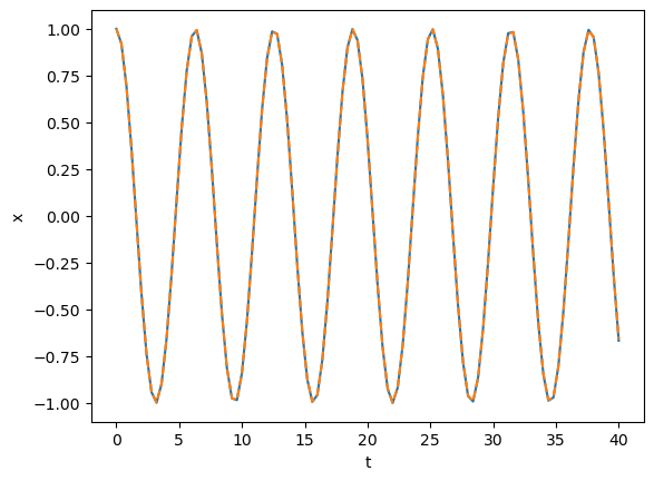
Let’s use Numba to accelerate RK4
import matplotlib.pyplot as plt
x_max = 1  # Size of x max
v_0 = 0
koverm = 1  # k / m


def f(t, y):
    "Y has two elements, x and v"
    return np.array([-koverm * y[1], y[0]])
def rk4_ivp(f, init_y, t):
    steps = len(t)
    order = len(init_y)

    y = np.empty((steps, order))
    y[0] = init_y

    for n in range(steps - 1):
        h = t[n + 1] - t[n]

        k1 = h * f(t[n], y[n])  # 2.1
        k2 = h * f(t[n] + h / 2, y[n] + k1 / 2)  # 2.2
        k3 = h * f(t[n] + h / 2, y[n] + k2 / 2)  # 2.3
        k4 = h * f(t[n] + h, y[n] + k3)  # 2.4

        y[n + 1] = y[n] + 1 / 6 * (k1 + 2 * k2 + 2 * k3 + k4)  # 2.0

    return y
ts = np.linspace(0, 40, 100 + 1)
y = rk4_ivp(f, [x_max, v_0], ts)
plt.plot(ts, np.cos(ts))
plt.plot(ts, y[:, 0], "--")
plt.xlabel("t")
plt.ylabel("x")
plt.show()
%%timeit
ts = np.linspace(0, 40, 1000 + 1)
y = rk4_ivp(f, [x_max, v_0], ts)
27.6 ms ± 655 µs per loop (mean ± std. dev. of 7 runs, 10 loops each)
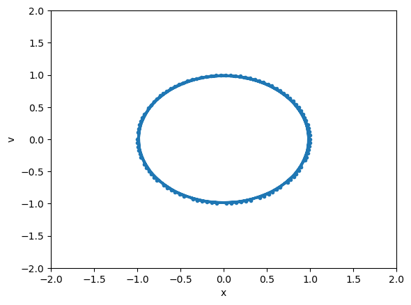
Animation#
import matplotlib
from matplotlib.animation import FuncAnimation

# First set up the figure, the axis, and the plot element we want to animate
fig = plt.figure()
ax = plt.axes(xlim=(-2, 2), ylim=(-2, 2), xlabel="x", ylabel="v")
line, = ax.plot([], [], lw=2, marker=".")

# initialization function: plot the background of each frame
def init():
    line.set_data([], [])
    return line,

# animation function.  This is called sequentially
# in this case, we will plot the solution from t=0 to the current time step
def animate(i):
    line.set_data(y[0:i+1, 0], y[0:i+1, 1])
    return line,

# call the animator.  blit=True means only re-draw the parts that have changed.
anim = FuncAnimation(fig, animate, init_func=init,
                     frames=len(y), interval=20, blit=True)

# save the animation as an mp4.  This requires ffmpeg or mencoder to be
# installed.  The extra_args ensure that the x264 codec is used, so that
# the video can be embedded in html5.  You may need to adjust this for
# your system: for more information, see
# http://matplotlib.sourceforge.net/api/animation_api.html
anim.save('basic_animation.mp4', fps=30, extra_args=['-vcodec', 'libx264'])
# Display .mp4 video
from IPython.display import Video
Video(data="basic_animation.mp4")
# Note we can also save it as a .gif
from IPython.display import Image
anim.save("basic_animation.gif", fps=30, writer="imagemagick")
Image(open("basic_animation.gif", "rb").read())