Lecture 03: Numerical Integration Methods#
Credit: https://pythonnumericalmethods.berkeley.edu/notebooks/Index.html
Euler Method#
Let \(\frac{dS(t)}{dt} = F(t,S(t))\) be an explicitly defined first order ODE. That is, \(F\) is a function that returns the derivative, or change, of a state given a time and state value. Also, let \(t\) be a numerical grid of the interval \([t_0, t_f]\) with spacing \(h\). Without loss of generality, we assume that \(t_0 = 0\), and that \(t_f = Nh\) for some positive integer, \(N\).
The linear approximation of \(S(t)\) around \(t_j\) at \(t_{j+1}\) is
which can also be written
This formula is called the Explicit Euler Formula, and it allows us to compute an approximation for the state at \(S(t_{j+1})\) given the state at \(S(t_j)\). Starting from a given initial value of \(S_0 = S(t_0)\), we can use this formula to integrate the states up to \(S(t_f)\); these \(S(t)\) values are then an approximation for the solution of the differential equation. The explicit Euler formula is the simplest and most intuitive method for solving initial value problems. At any state \((t_j, S(t_j))\) it uses \(F\) at that state to “point” toward the next state and then moves in that direction a distance of \(h\). Although there are more sophisticated and accurate methods for solving these problems, they all have the same fundamental structure. As such, we enumerate explicitly the steps for solving an initial value problem using the Explicit Euler formula.

WHAT IS HAPPENING? Assume we are given a function \(F(t, S(t))\) that computes \(\frac{dS(t)}{dt}\), a numerical grid, \(t\), of the interval, \([t_0, t_f]\), and an initial state value \(S_0 = S(t_0)\). We can compute \(S(t_j)\) for every \(t_j\) in \(t\) using the following steps.
Store \(S_0 = S(t_0)\) in an array, \(S\).
Compute \(S(t_1) = S_0 + hF(t_0, S_0)\).
Store \(S_1 = S(t_1)\) in \(S\).
Compute \(S(t_2) = S_1 + hF(t_1, S_1)\).
Store \(S_2 = S(t_1)\) in \(S\).
\(\cdots\)
Compute \(S(t_f) = S_{f-1} + hF(t_{f-1}, S_{f-1})\).
Store \(S_f = S(t_f)\) in \(S\).
\(S\) is an approximation of the solution to the initial value problem.
When using a method with this structure, we say the method integrates the solution of the ODE.
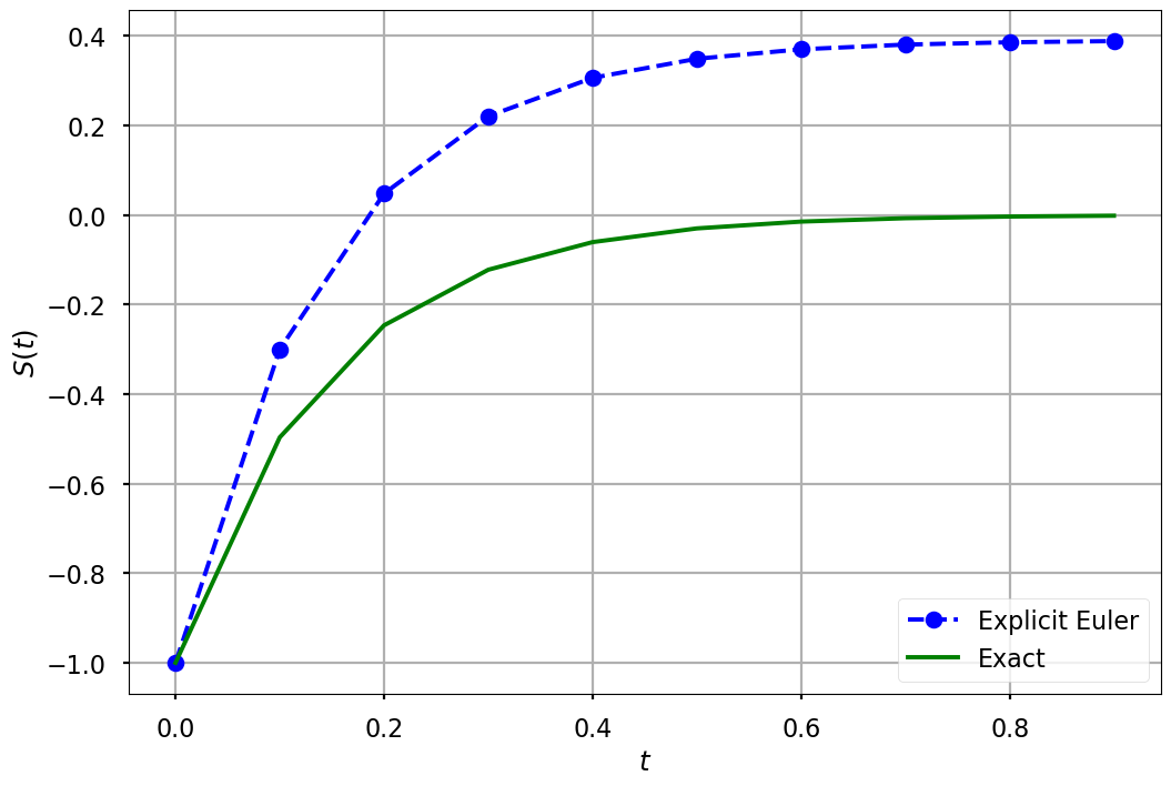
Example: The differential equation \(\frac{df(t)}{dt} = e^{-t}\) with initial condition \(f_0 = -1\) has the exact solution \(f(t) = -e^{-t}\). Approximate the solution to this initial value problem between 0 and 1 in increments of 0.1 using the explicit Euler Formula. Plot the difference between the approximated solution and the exact solution.
import numpy as np
import matplotlib.pyplot as plt

%matplotlib inline

plt.style.use('seaborn-poster')
# Define parameters
f = lambda t, s: 7*np.exp(-7*t) # ODE
g = lambda t: -np.exp(-7*t) # Exact solution

h = 0.1 # Step size
t = np.arange(0, 10*h, h) # Numerical grid
s0 = -1 # Initial condition
/tmp/ipykernel_4501/3962005646.py:6: MatplotlibDeprecationWarning: The seaborn styles shipped by Matplotlib are deprecated since 3.6, as they no longer correspond to the styles shipped by seaborn. However, they will remain available as 'seaborn-v0_8-<style>'. Alternatively, directly use the seaborn API instead.
  plt.style.use('seaborn-poster')
# Explicit Euler method
s = np.zeros(len(t))
s_imp = np.zeros(len(t))
s[0] = s0
s_imp[0] = s0


for i in range(0, len(t) - 1):
    s[i + 1] = s[i] + h*f(t[i], s[i])
    s_imp[i + 1] = s[i] + h*f(t[i+1], s[i+1])

plt.figure(figsize = (12, 8))
plt.plot(t, s, 'bo--', label='Explicit Euler')
plt.plot(t, g(t), 'g', label='Exact')
plt.xlabel('$t$')
plt.ylabel('$S(t)$')
plt.grid()
plt.legend(loc='lower right')
plt.savefig("explicit_euler.pdf")
plt.show()
The explicit Euler Formula is called “explicit” because it only requires information at \(t_j\) to compute the state at \(t_{j+1}\). That is, \(S(t_{j+1})\) can be written explicitly in terms of values we have (i.e., \(t_j\) and \(S(t_j)\)). The implicit Euler formula can be derived by taking the linear approximation of \(S(t)\) around \(t_{j+1}\) and computing it at \(t_j\):
This formula is peculiar because it requires that we know \(S(t_{j+1})\) to compute \(S(t_{j+1})\)! However, it happens that sometimes we can use this formula to approximate the solution to initial value problems.
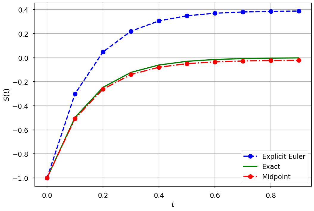
Midpoint method#
# Explicit Midpoint method
s_mid = np.zeros(len(t))
s_mid[0] = s0

for i in range(0, len(t) - 1):
    s_mid[i + 1] = s_mid[i] + h*f(t[i] + h/2, s_mid[i] + (h/2)*f(t[i], s_mid[i]))

plt.figure(figsize = (12, 8))
plt.plot(t, s, 'bo--', label='Explicit Euler')
plt.plot(t, g(t), 'g', label='Exact')
plt.plot(t, s_mid, 'ro-.', label='Midpoint')
plt.xlabel('$t$')
plt.ylabel('$S(t)$')
plt.grid()
plt.legend(loc='lower right')
plt.savefig("explicit_euler_midpoint.pdf")
plt.show()
Predictor-Corrector Methods#
Given any time and state value, the function, \(F(t, S(t))\), returns the change of state \(\frac{dS(t)}{dt}\). Predictor-corrector methods of solving initial value problems improve the approximation accuracy by querying the \(F\) function several times at different locations (predictions), and then using a weighted average of the results (corrections) to update the state. Essentially, it uses two formulas: the predictor and corrector. The predictor is an explicit formula and first estimates the solution at \(t_{j+1}\), i.e. we can use Euler method or some other methods to finish this step. After we obtain the solution \(S(t_{j+1})\), we can apply the corrector to improve the accuracy. Using the found \(S(t_{j+1})\) on the right-hand side of an otherwise implicit formula, the corrector can calculate a new, more accurate solution.
The midpoint method has a predictor step:
which is the prediction of the solution value halfway between \(t_j\) and \(t_{j+1}\).
It then computes the corrector step:
which computes the solution at \(S(t_{j+1})\) from \(S(t_j)\) but using the derivative from \(S\left(t_{j} + \frac{h}{2}\right)\).
Runge-Kutta Methods#
Runge Kutta (RK) methods are one of the most widely used methods for solving ODEs. Recall that the Euler method uses the first two terms in Taylor series to approximate the numerical integration, which is linear: \(S(t_{j+1}) = S(t_j + h) = S(t_j) + h \cdot S'(t_j)\).
We can greatly improve the accuracy of numerical integration if we keep more terms of the series in
In order to get this more accurate solution, we need to derive the expressions of \(S''(t_j), S'''(t_j), \cdots, S^{(n)}(t_j)\). This extra work can be avoided using the RK methods, which is based on truncated Taylor series, but not require computation of these higher derivatives.
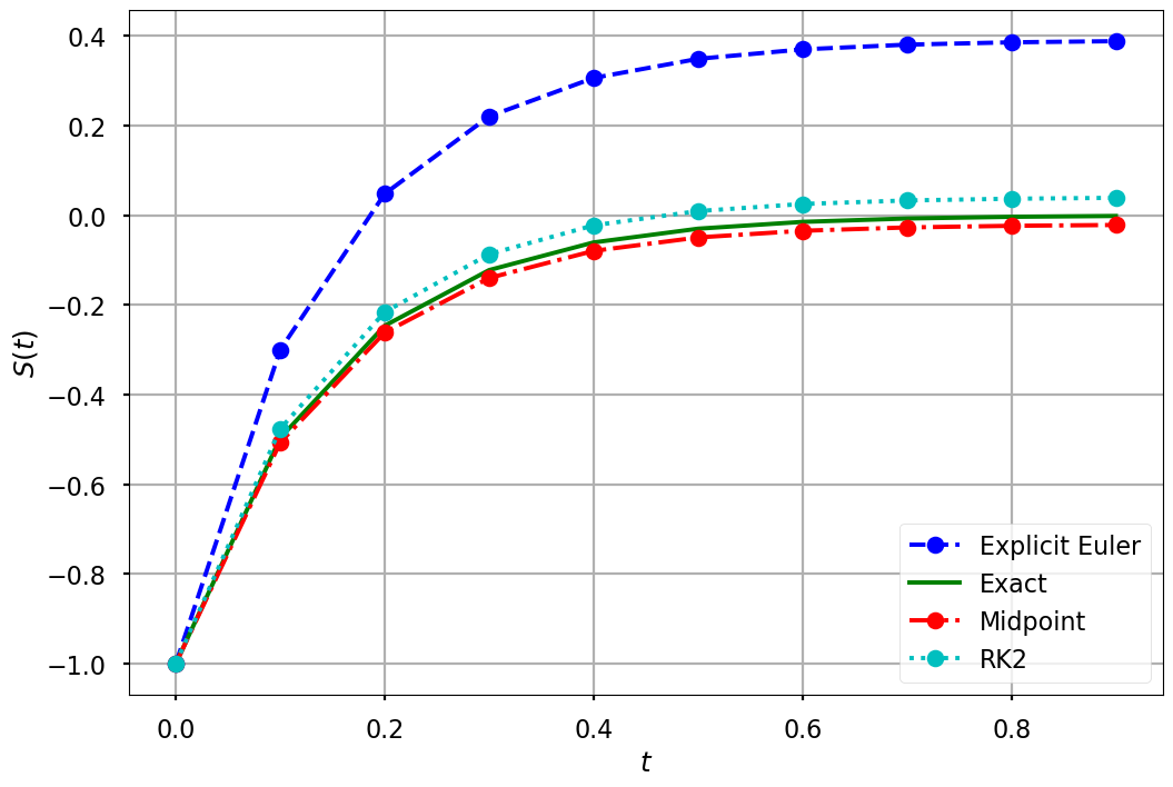
Second-order Runge-Kutta method#
Let us first derive the second-order RK method. Let \(\frac{dS(t)}{dt} = F(t,S(t))\), then we can assume an integration formula the form of
We can attempt to find these parameters \(c_1, c_2, p, q\) by matching the above equation to the second-order Taylor series, which gives us
Noting that
Therefore, this equation can be written as:
We can also rewrite the last term by applying Taylor series in several variables, which gives us:
thus the equation becomes:
Comparing equations, we can easily obtain:
Because the equation has four unknowns and only three equations, we can assign any value to one of the parameters and get the rest of the parameters. One popular choice is:
We can also define: $\( \begin{align} k_1 & = F(t_j,S(t_j))\\ k_2 & = F\left(t_j+ph, S(t_j)+qhk_1\right) \end{align} \)$
where we will have:
# RK2 method
s_rk2 = np.zeros(len(t))
s_rk2[0] = s0

for i in range(0, len(t) - 1):

    k1 = f(t[i], s_rk2[i])
    k2 = f(t[i] + h, s_rk2[i] + h*k1 )
    s_rk2[i + 1] = s_rk2[i] + (h/2)*(k1+k2)

plt.figure(figsize = (12, 8))
plt.plot(t, s, 'bo--', label='Explicit Euler')
plt.plot(t, g(t), 'g', label='Exact')
plt.plot(t, s_mid, 'ro-.', label='Midpoint')
plt.plot(t, s_rk2, 'co:', label='RK2')
plt.xlabel('$t$')
plt.ylabel('$S(t)$')
plt.grid()
plt.legend(loc='lower right')
plt.savefig("explicit_euler_midpoint_rk2.pdf")
plt.show()
Fourth-order Runge-Kutta method#
A classical method for integrating ODEs with a high order of accuracy is the Fourth-order Runge-Kutta (RK4) method. It is obtained from the Taylor series using similar approach we just discussed in the second-order method. This method uses four points \(k_1, k_2, k_3\), and \(k_4\). A weighted average of these is used to produce the approximation of the solution. The formula is as follows.
Therefore, we will have:
As indicated by its name, the RK4 method is fourth-order accurate, or \(O(h^4)\).
# RK4 method
s_rk4 = np.zeros(len(t))
s_rk4[0] = s0
for i in range(0, len(t) - 1):
k1 = f(t[i], s_rk4[i])
k2 = f(t[i] + h/2, s_rk4[i] + h*k1/2 )
k3 = f(t[i] + h/2, s_rk4[i] + h*k2/2 )
k4 = f(t[i] + h, s_rk4[i] + h*k3)
s_rk4[i + 1] = s_rk4[i] + (h/6)*(k1+2*k2 + 2*k3 + k4)
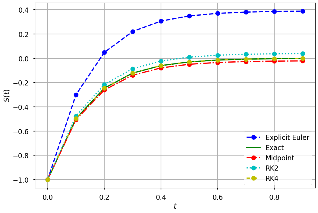
plt.figure(figsize = (12, 8))
plt.plot(t, s, 'bo--', label='Explicit Euler')
plt.plot(t, g(t), 'g', label='Exact')
plt.plot(t, s_mid, 'ro-.', label='Midpoint')
plt.plot(t, s_rk2, 'co:', label='RK2')
plt.plot(t, s_rk4, 'oy', ls=(0, (3, 5, 1, 5, 1, 5)), label='RK4')
plt.xlabel('$t$')
plt.ylabel('$S(t)$')
plt.grid()
plt.legend(loc='lower right')
plt.savefig("explicit_euler_midpoint_rk4.pdf")
plt.show()