
Lab 1: Introduction#
Some helpful links:
Python (https://docs.python.org/3.9/tutorial/index.html): an introduction to the Python programming language
Google Colab (https://colab.research.google.com/): for Python development in your web-browser
Miniconda (https://docs.conda.io/en/latest/miniconda.html): a free minimal installer for conda
NumPy (https://numpy.org/doc/stable/user/quickstart.html): a widely used library for mathematical operations in Python
Seaborn (https://seaborn.pydata.org/): a library for creating nice looking graphs and figures
NumPy array basics#
The basic data structure is a NumPy array
# Import NumPy
import numpy as np
# Define a 1D array (i.e. a vector)
x = np.array([1, 2, 3, 4])
# Check the "shape" of the array
x.shape
(4,)
# Define a 2D array (i.e. a matrix)
w = np.array([[1, 2, 3, 4],
              [1, 2, 3, 4]])
# Check the shape of w
w.shape
(2, 4)
# Do a matrix multiplication
out = np.matmul(w, x)
# Note, this is the same
out = w @ x
print(out)
[30 30]
out.shape
(2,)
Loading data with Numpy#
data = np.loadtxt(fname="data/leapfrog_sho.txt")

print(data)
[[ 0.        0.        1.        0.      ]
 [ 0.125     0.        0.992197 -0.124665]
 [ 0.25      0.        0.96891  -0.247384]
 [ 0.375     0.        0.930502 -0.366242]
 [ 0.5       0.        0.877573 -0.479385]
 [ 0.625     0.        0.810948 -0.585046]
 [ 0.75      0.        0.731668 -0.681578]
 [ 0.875     0.        0.64097  -0.767473]
 [ 1.        0.        0.540268 -0.84139 ]
 [ 1.125     0.        0.431135 -0.902177]
 [ 1.25      0.        0.315274 -0.948885]
 [ 1.375     0.        0.194493 -0.980784]
 [ 1.5       0.        0.070676 -0.997378]
 [ 1.625     0.       -0.054243 -0.998406]
 [ 1.75      0.       -0.178316 -0.983853]
 [ 1.875     0.       -0.299606 -0.953946]
 [ 2.        0.       -0.416221 -0.909153]
 [ 2.125     0.       -0.52634  -0.85017 ]
 [ 2.25      0.       -0.628245 -0.777921]
 [ 2.375     0.       -0.720346 -0.693531]
 [ 2.5       0.       -0.801204 -0.598318]
 [ 2.625     0.       -0.86956  -0.493767]
 [ 2.75      0.       -0.924345 -0.381511]
 [ 2.875     0.       -0.964705 -0.263301]
 [ 3.        0.       -0.99001  -0.140982]
 [ 3.125     0.       -0.999864 -0.016463]
 [ 3.25      0.       -0.994115  0.108313]
 [ 3.375     0.       -0.972852  0.231399]
 [ 3.5       0.       -0.936407  0.350874]
 [ 3.625     0.       -0.885348  0.464873]
 [ 3.75      0.       -0.820472  0.571617]
 [ 3.875     0.       -0.742792  0.66944 ]
 [ 4.        0.       -0.65352   0.756816]
 [ 4.125     0.       -0.55405   0.832382]
 [ 4.25      0.       -0.445933  0.894957]
 [ 4.375     0.       -0.330856  0.943566]
 [ 4.5       0.       -0.210617  0.977449]
 [ 4.625     0.       -0.08709   0.996079]
 [ 4.75      0.        0.037795  0.999164]
 [ 4.875     0.        0.162091  0.986655]
 [ 5.        0.        0.283857  0.958749]
 [ 5.125     0.        0.401194  0.915881]
 [ 5.25      0.        0.512269  0.85872 ]
 [ 5.375     0.        0.61535   0.788158]
 [ 5.5       0.        0.708828  0.705296]
 [ 5.625     0.        0.791244  0.611426]
 [ 5.75      0.        0.861311  0.508016]
 [ 5.875     0.        0.917938  0.396676]
 [ 6.        0.        0.960238  0.279147]
 [ 6.125     0.        0.987554  0.157261]
 [ 6.25      0.        0.999458  0.032921]
 [ 6.375     0.        0.995764 -0.091933]
 [ 6.5       0.        0.976531 -0.215352]
 [ 6.625     0.        0.942058 -0.33541 ]
 [ 6.75      0.        0.892883 -0.450234]
 [ 6.875     0.        0.829774 -0.558032]
 [ 7.        0.        0.753715 -0.657121]
 [ 7.125     0.        0.665894 -0.745955]
 [ 7.25      0.        0.567681 -0.823148]
 [ 7.375     0.        0.460609 -0.887495]
 [ 7.5       0.        0.346349 -0.937991]
 [ 7.625     0.        0.226684 -0.97385 ]
 [ 7.75      0.        0.103481 -0.99451 ]
 [ 7.875     0.       -0.021337 -0.99965 ]
 [ 8.        0.       -0.145822 -0.98919 ]]
The expression np.loadtxt(...) is a function call that asks Python to run the function] loadtxt that
belongs to the NumPy library.
The dot notation in Python is used most of all as an object attribute/property specifier or for invoking its method.
object.property will give you the object.property value, object_name.method() will invoke on object_name method.
np.loadtxt has two parameters: the name of the file we want to read and the delimiter that separates values on a line.
These both need to be character strings (or strings for short), so we put them in quotes.
By default, only a few rows and columns are shown (with ... to omit elements when displaying big arrays).
Note that, to save space when displaying NumPy arrays, Python does not show us trailing zeros, so 1.0 becomes 1..
# Let's print out some features of this data
print(type(data))
print(data.dtype)
print(data.shape)
<class 'numpy.ndarray'>
float64
(65, 4)
The output tells us that the data array variable contains 65 rows and 4 columns.
When we created the variable data to store our data, we did not only create the array; we also created information about the array, called members or attributes.
data.shape is an attribute of data which describes the dimensions of data.
If we want to get a single number from the array, we must provide an index in square brackets after the variable name, just as we do in math when referring to an element of a matrix.
Our data has two dimensions, so we will need to use two indices to refer to one specific value:
print(f"first value in data: {data[0, 0]}")
first value in data: 0.0
print(f"middle value in data: {data[30, 0]}")
middle value in data: 3.75
The expression data[30, 0] accesses the element at row 30, column 0, while data[0, 0] accesses the element at row 0, column 0.
Languages in the C family (including C++, Java, Perl, and Python) count from 0 because it represents an offset from the first value in the array (the second value is offset by one index from the first value).
As a result, if we have an \(M\times N\) array in Python, its indices go from \(0\) to \(M-1\) on the first axis and \(0\) to \(N-1\) on the second.
!["data" is a 3 by 3 numpy array containing row 0: ['A', 'B', 'C'], row 1: ['D', 'E', 'F'], androw 2: ['G', 'H', 'I']. Starting in the upper left hand corner, data[0, 0] = 'A', data[0, 1] = 'B', data[0, 2] = 'C', data[1, 0] = 'D', data[1, 1] = 'E', data[1, 2] = 'F', data[2, 0] = 'G', data[2, 1] = 'H', and data[2, 2] = 'I', in the bottom right hand corner.](../../_images/python-zero-index.svg)
When Python displays an array, it shows the element with index [0, 0] in the upper left corner rather than the lower left.
This is consistent with the way mathematicians draw matrices but different from the Cartesian coordinates.
The indices are (row, column) instead of (column, row) for the same reason, which can be confusing when plotting data.
Slicing data#
An index like [30, 0] selects a single element of an array, but we can select whole sections as well.
print(data[0:4, :])
[[ 0.        0.        1.        0.      ]
 [ 0.125     0.        0.992197 -0.124665]
 [ 0.25      0.        0.96891  -0.247384]
 [ 0.375     0.        0.930502 -0.366242]]
The slice 0:4 means, “Start at index 0 and go up to, but not including, index 4”.
The difference between the upper and lower bounds is the number of values in the slice.
We don’t have to start slices at 0:
print(data[5:10, :])
[[ 0.625     0.        0.810948 -0.585046]
 [ 0.75      0.        0.731668 -0.681578]
 [ 0.875     0.        0.64097  -0.767473]
 [ 1.        0.        0.540268 -0.84139 ]
 [ 1.125     0.        0.431135 -0.902177]]
We also don’t have to include the upper and lower bound on the slice.
If we don’t include the lower bound, Python uses 0 by default; if we don’t include the upper, the slice runs to the end of the axis, and if we don’t include either (i.e., if we use : on its own), the slice includes everything:
small = data[:3, 2:]
print(f"small is:\n{small}")
small is:
[[ 1.        0.      ]
 [ 0.992197 -0.124665]
 [ 0.96891  -0.247384]]
The above example selects rows 0 through 2 and columns 2 through to the end of the array.
Analyzing data#
NumPy has several useful functions that take an array as input to perform operations on its values.
If we want to find the average inflammation for all patients on
all days, for example, we can ask NumPy to compute data’s mean value:
np.mean(data)
np.float64(0.9949353961538463)
However, this is not very meaningful because it’s a mean over positions, velocities, etc. Instead, we can ask for the average position (or velocity) over all time steps.
# average position
print(np.mean(data[:, 2]))

# average velocity
print(np.mean(data[:, 3]))
0.1281684307692308
-0.14842684615384616
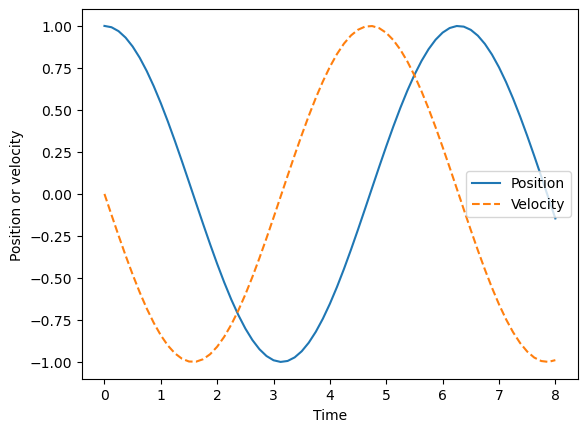
Visualizing data#
Visualization deserves an entire lecture of its own, but we can explore a few features of Python’s matplotlib library here.
While there is no official plotting library, matplotlib is the de facto standard.
First, we will import the pyplot module from matplotlib and use it to create and display our data:
import matplotlib.pyplot as plt

plt.plot(data[:, 0], data[:, 2], label="Position")
plt.plot(data[:, 0], data[:, 3], label="Velocity", ls="--")

plt.ylabel("Position or velocity")
plt.xlabel("Time")

plt.legend()

plt.show()
Make your own plot#
Create a plot showing the position, velocity, and acceleration of the point at each time step.
# Your code here