Lab 8: Assignment 2 Tutorial

Consider the double potential well,

\[V(x) = \alpha x^4 - 2x^2 + + \frac{1}{\alpha}\]

where \(x\) is the position of the particle, and we set \(m=\hbar=1\). For parts 1A, 1B, and 1C, you may set \(\alpha = 0.4\). For the last part, you will need to vary \(\alpha\). The minima of the potential are at \(x_\mathrm{min}^2 = \pm\frac{1}{\alpha}\) and the barrier height is \(V(0) = \frac{1}{\alpha}\).

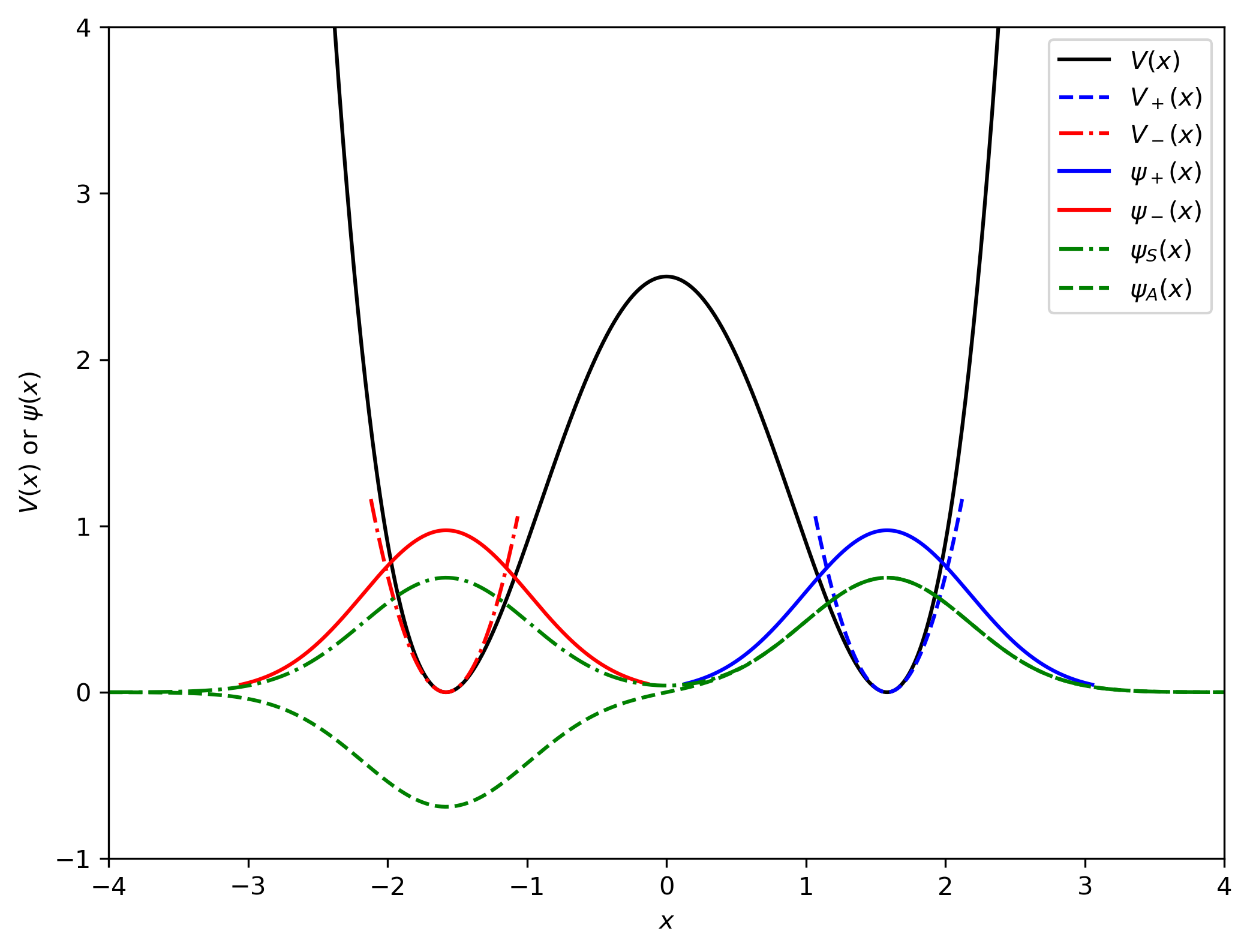
As discussed in lecture 9, we can approximate the potential by a harmonic potential near the minima.

\[V_+(x) = 4(x-x_\mathrm{min})^2\]

\[V_-(x) = 4(x+x_\mathrm{min})^2,\]

which implies \(\omega = 2\sqrt{2}\). The ground state wave functions for those approximate potential wells are

\[\psi_+(x) = \left(\frac{\omega}{\pi}\right)^{1/4} \exp\left(- \frac{\omega}{2}(x-x_\mathrm{min})^2\right)\]

\[\psi_-(x) = \left(\frac{\omega}{\pi}\right)^{1/4} \exp\left(- \frac{\omega}{2}(x+x_\mathrm{min})^2\right)\]

We can approximate the ground state and first excited state as the symmetric and antisymmetric combinations of these wave functions, respectively.

\[\psi_0(x) \approx \psi_\mathrm{S}(x) = \frac{1}{\sqrt{2}}\left ( \psi_+(x) + \psi_-(x) \right )\]

\[\psi_1(x) \approx \psi_\mathrm{A}(x) = \frac{1}{\sqrt{2}}\left ( \psi_+(x) - \psi_-(x) \right )\]

The energy gap between the ground state and first excited state is \(\Delta E = E_1 - E_0\).

Problem 1A

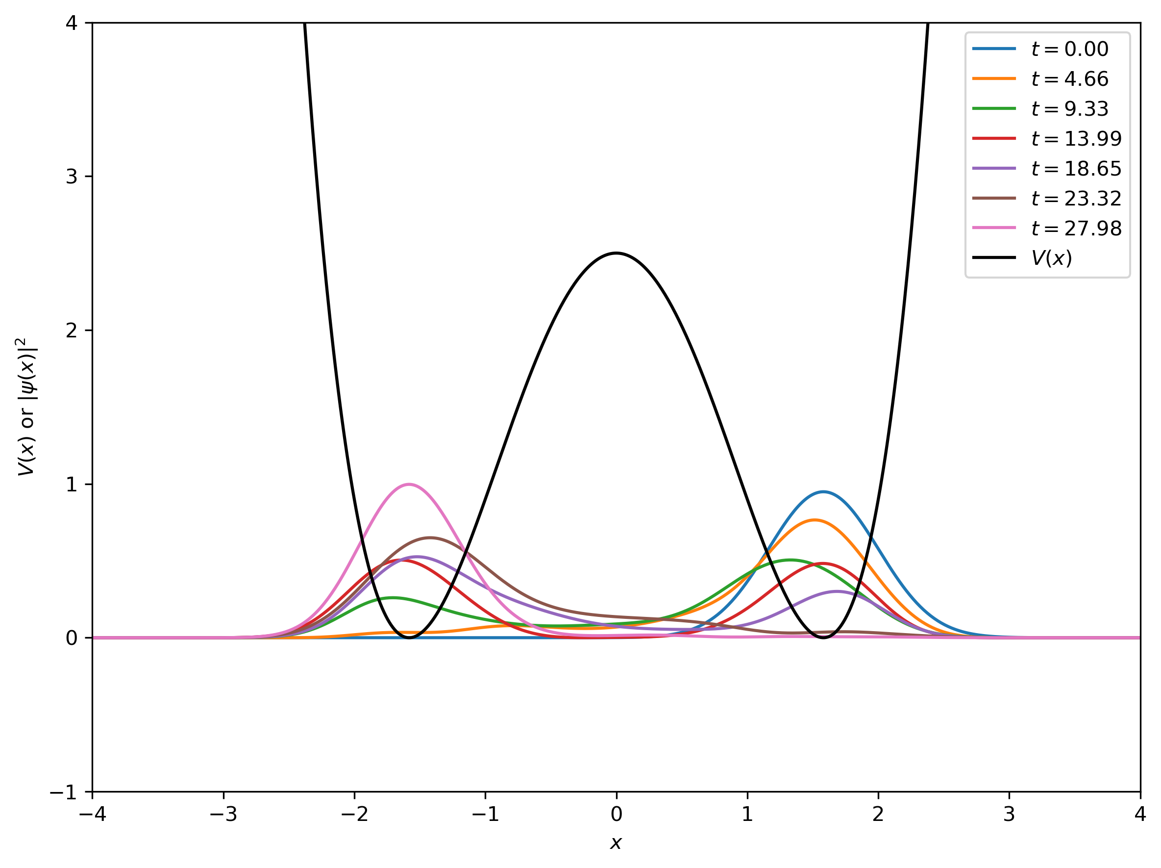
Demonstrate tunneling between the two wells using the Feynman path integral. Start with the particle in the right well $\( \psi(x, 0) = \psi_+(x), \)$ and evolve the wave function at each time step using the elementary propagator.

Numerically, you may use discretization parameters similar to Assignment 1: \(\epsilon = \Delta t = \pi/128\), \(x_0 = -4\), \(x_{N_D} = +4\), and \(N_D=600\). You will have to simulate a long enough period \(T > t_\mathrm{tunnel}\) that is longer than the tunneling time. As a reminder, the tunneling time is defined as the time it takes for the particle to reach the left well.

Plot the mean position \(\langle x \rangle\) as a function of time \(t\). How can you estimate the tunneling time \(t_\mathrm{tunnel}\) from this plot?

Hint: You may approximate the propagator as

\[\tilde {\mathcal K}(x_b, \epsilon; x_a, 0) \sim \exp \left( i\left( \frac{1}{2}\frac{(x_b - x_a)^2}{\epsilon} - V\left(\frac{x_a+x_b}{2}\right) \epsilon \right)\right),\]

where \(x_a\) and \(x_b\) are the initial and final positions, respectively, and \(\epsilon\) is the time step. Note, we lack the normalization factor in this approximation so you will need to normalize the wave function at each time step

\[\psi(x, t) \leftarrow \frac{\psi(x, t)}{\sqrt{\int_{-\infty}^{\infty} |\psi(x, t)|^2 dx}}.\]

import matplotlib.pyplot as plt
import numpy as np

ALPHA = 0.4
XMIN = np.sqrt(1 / ALPHA)
OMEGA = np.sqrt(8 * ALPHA * XMIN ** 2)
XSTART = XMIN
BOXSIZE = 8
ND = 600
DELTAX = BOXSIZE / ND
HBAR = 1
T0 = 20 * np.pi
DELTAT = np.pi / 128
NT = int(T0 / DELTAT)

t = np.linspace(0, T0, NT + 1)
x = np.linspace(-BOXSIZE / 2, BOXSIZE / 2, ND + 1)

def V(x):
    return -2*x**2 + ALPHA*x**4 + 1/ALPHA

def V_plus(x):
    return 4*(x-1/np.sqrt(ALPHA))**2

def V_minus(x):
    return 4*(x+1/np.sqrt(ALPHA))**2

def func_psi_0(x, x_start):
    part1 = (OMEGA / np.pi) ** (1 / 4)
    part2 = np.exp(-( OMEGA / (2 * HBAR)) * (x - x_start)**2)
    return part1 * part2

psi_plus = func_psi_0(x, XMIN) 
psi_minus = func_psi_0(x, -XMIN)
psi_A = (psi_plus - psi_minus)/np.sqrt(2)
psi_S = (psi_plus + psi_minus)/np.sqrt(2)

plt.figure(dpi=300, figsize=(8,6))
plt.plot(x, V(x), 'k-', label=r'$V(x)$')
plt.plot(x[380:460], V_plus(x[380:460]), 'b--', label=r'$V_+(x)$')
plt.plot(x[-460:-380], V_minus(x[-460:-380]), 'r-.', label=r'$V_-(x)$')
plt.plot(x[310:530], psi_plus[310:530], 'b-', label=r'$\psi_+(x)$')
plt.plot(x[-530:-310], psi_minus[-530:-310], 'r-', label=r'$\psi_-(x)$')
plt.plot(x, psi_S, 'g-.', label=r'$\psi_S(x)$')
plt.plot(x, psi_A, 'g--', label=r'$\psi_A(x)$')
plt.ylabel(r'$V(x)$ or $\psi(x)$')
plt.xlabel(r'$x$')
plt.xlim(-4, 4)
plt.ylim(-1, 4)
plt.legend()
plt.savefig("V_all.pdf")
plt.show()

def func_K(x_a, x_b, dt):
    exponent = 1j * (0.5 * (x_b - x_a)**2 / dt - V((x_a + x_b) / 2) * dt)
    return np.exp(exponent)

K_dt = np.zeros((ND + 1, ND + 1), dtype=np.complex64)
for i in range(ND + 1):
    for j in range(ND + 1):
        K_dt[i, j] = func_K(x[i], x[j], DELTAT)

psi_0 = func_psi_0(x, XSTART) 

print("Check normalization: ", np.sum(psi_0 * psi_0.conjugate()) * DELTAX)

Check normalization:  0.9999999960164199

psi = [psi_0]

for i in range(1, NT + 1):
    psi_t = DELTAX * np.matmul(K_dt, psi[i-1])
    # normalize to 1
    psi_t /= np.sqrt(DELTAX * np.sum(psi_t * psi_t.conjugate()))
    psi.append(psi_t)

prob = []
for i in range(NT + 1):
    prob.append(np.real(psi[i] * psi[i].conjugate()))

x_bar = np.zeros_like(t)
for i in range(NT + 1):
    x_bar[i] = sum(prob[i] * x * DELTAX)

plt.figure(figsize=(6, 6))
plt.plot(t, x_bar)
plt.xlabel(r"$t$")
plt.ylabel(r"$\langle x \rangle$")
plt.show()

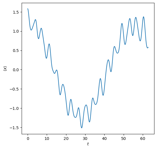
# approximate tunneling time
t[np.argmin(x_bar)]

np.float64(28.151615419277288)

plot_interval = 190
xmin, xmax, ymin, ymax = -BOXSIZE/2, BOXSIZE/2, -1, 4
plt.figure(dpi=300, figsize=(8, 6))
for i in range(0, NT // 2 + 1, plot_interval):
    plt.plot(x, prob[i].real, label=f"$t = {i * DELTAT:.2f}$")
plt.plot(x, V(x), 'k', label='$V(x)$')
plt.xlabel("$x$")
plt.ylabel("$V(x)$ or $|\psi(x)|^2$")
plt.xlim([xmin, xmax])
plt.ylim([ymin, ymax])
plt.legend(loc='upper right')
plt.tight_layout()
plt.show()