Lecture 10: Eigenvalue Problem Demo

import matplotlib.pyplot as plt
import numpy as np
import scipy

OMEGA = 1
BOXSIZE = 8
ND = 600
DELTAX = BOXSIZE / ND
HBAR = 1

x = np.linspace(-BOXSIZE / 2, BOXSIZE / 2, ND + 1)

def V(x):
    return 0.5*x**2

H = np.zeros((ND + 1, ND + 1))

for i in range(ND + 1):
    for j in range(ND + 1):
        # kinetic part
        H[i, j] = -(0.5 / DELTAX**2) * ((i + 1 == j) - 2 * (i == j) + (i - 1 == j)) 
        # potential part
        H[i, j] += V(x[i]) * (i == j)

# print the first 4x4 elements of H
print(H[:4,:4])

[[ 5633.         -2812.5            0.             0.        ]
 [-2812.5         5632.94675556 -2812.5            0.        ]
 [    0.         -2812.5         5632.89368889 -2812.5       ]
 [    0.             0.         -2812.5         5632.8408    ]]

%%timeit
# standard method
Es, psi = scipy.linalg.eigh(H)

40.1 ms ± 186 μs per loop (mean ± std. dev. of 7 runs, 10 loops each)

%%timeit
# find the lowest eigenvalues and corresponding eigenvectors of H using ARPACK
Es, psis = scipy.sparse.linalg.eigsh(H, k=2, which='SM')

410 ms ± 9.04 ms per loop (mean ± std. dev. of 7 runs, 1 loop each)

%%timeit
# shift-invert mode is faster for finding these
Es, psis = scipy.sparse.linalg.eigsh(H, k=2, sigma=0, which='LM')

6.24 ms ± 81.4 μs per loop (mean ± std. dev. of 7 runs, 100 loops each)

Es, psis = scipy.sparse.linalg.eigsh(H, k=2, sigma=0, which='LM')

E_0 = Es[0]
E_1 = Es[1]
psi_0 = psis[:, 0]
psi_1 = psis[:, 1]

# normalize the wave functions
psi_0 /= np.sqrt(np.sum(psi_0.conjugate() * psi_0) * DELTAX)
psi_1 /= np.sqrt(np.sum(psi_1.conjugate() * psi_1) * DELTAX)

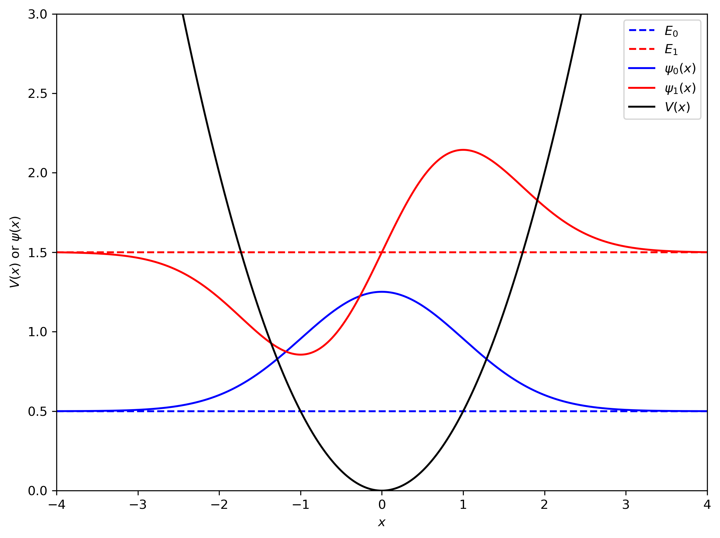
xmin, xmax, ymin, ymax = -BOXSIZE/2, BOXSIZE/2, 0, 3
plt.figure(dpi=300, figsize=(8, 6))
plt.plot(x, E_0*np.ones_like(x), 'b--', label=f"$E_0$")
plt.plot(x, E_1*np.ones_like(x), 'r--', label=f"$E_1$")
plt.plot(x, psi_0 + E_0, 'b-', label=f"$\psi_0(x)$")
plt.plot(x, psi_1 + E_1, 'r-', label=f"$\psi_1(x)$")
plt.plot(x, V(x), 'k', label='$V(x)$')
plt.xlabel("$x$")
plt.ylabel(r"$V(x)$ or $\psi(x)$")
plt.xlim([xmin, xmax])
plt.ylim([ymin, ymax])
plt.legend(loc='upper right')
plt.tight_layout()
plt.savefig("ho_e0_e1.pdf")
plt.show()