Lab 4: Free Particle Propagator (Assignment 1 Tutorial)

In assignment 1, we will perform the path integral numerically for the harmonic oscillator. In today’s lab, we’ll start with a simpler problem: the free particle.

\[L = K = \frac{1}{2}\dot{x}^2\]

where \(m = \hbar = 1\) in these units.

Setup

We will use the discrete approximation to the path integral over a time period \(T_0 = 2\pi\), where the time step is \(\epsilon = \Delta t = T_0/128\). The electron position is also discretized into \(N_D+1\) possible points, \(x_0 = -4, x_1, x_2, \ldots, x_{N_D} = +4\), where \(N_D=600\).

Let’s set these up as constants in our code.

import matplotlib.pyplot as plt
import numpy as np

T0 = 2 * np.pi 
NT = 128 
DELTAT = T0 / NT
BOXSIZE = 8
ND = 600
DELTAX = BOXSIZE / ND
HBAR = 1

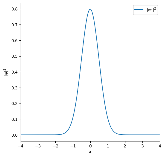
Initial probability amplitude

The initial probability amplitude (sometimes called the wavefunction) of the electron is a Gaussian centered at \(x_\mathrm{start}\),

\[\Psi_0(x) = \left(\frac{\alpha}{\pi}\right)^{1/4}\exp\left(-\frac{\alpha}{2}(x-x_\mathrm{start})^2\right),\]

where \(\alpha = 2\) and \(x_\mathrm{start} = 0\). The amplitude can be represented as a vector \(\psi_0\) with \(N_D+1\) components, \(\psi_0 = (\Psi_0(x_0), \Psi_0(x_1), \ldots, \Psi_0(x_{N_D}))\).

We will plot this initial amplitude and check it’s normalization.

XSTART = 0

t = np.linspace(0, T0, NT + 1)
x = np.linspace(-BOXSIZE / 2, BOXSIZE / 2, ND + 1)

def func_psi_0(x, x_start):
    alpha = 2
    return (alpha / np.pi) ** (1 / 4) * np.exp(-alpha / 2 * (x - x_start)**2)

psi_0 = func_psi_0(x, XSTART)

print(f"Psi at every 10th point: {psi_0[::10]}")
print(f"Normalization condition:  {DELTAX * sum(psi_0 * psi_0.conjugate())}")

Psi at every 10th point: [1.00521352e-07 2.86935958e-07 7.90442079e-07 2.10142331e-06
 5.39157259e-06 1.33498316e-05 3.19002830e-05 7.35650786e-05
 1.63722093e-04 3.51642446e-04 7.28876109e-04 1.45802361e-03
 2.81471103e-03 5.24398563e-03 9.42860819e-03 1.63603316e-02
 2.73964970e-02 4.42747775e-02 6.90519833e-02 1.03933211e-01
 1.50970103e-01 2.11634261e-01 2.86311914e-01 3.73810316e-01
 4.71000711e-01 5.72730433e-01 6.72105390e-01 7.61172192e-01
 8.31930157e-01 8.77504273e-01 8.93243842e-01 8.77504273e-01
 8.31930157e-01 7.61172192e-01 6.72105390e-01 5.72730433e-01
 4.71000711e-01 3.73810316e-01 2.86311914e-01 2.11634261e-01
 1.50970103e-01 1.03933211e-01 6.90519833e-02 4.42747775e-02
 2.73964970e-02 1.63603316e-02 9.42860819e-03 5.24398563e-03
 2.81471103e-03 1.45802361e-03 7.28876109e-04 3.51642446e-04
 1.63722093e-04 7.35650786e-05 3.19002830e-05 1.33498316e-05
 5.39157259e-06 2.10142331e-06 7.90442079e-07 2.86935958e-07
 1.00521352e-07]
Normalization condition:  0.9999999999999982

Exercise 1: Plot the initial probability distribution

xmin, xmax = -BOXSIZE / 2, BOXSIZE / 2
plt.figure(figsize=(6, 6))
# plot the initial probability distribution here
plt.plot(x, psi_0 * psi_0.transpose(), label=r"$|\psi_0|^2$")
plt.xlabel(r"$x$")
plt.ylabel(r"$|\psi|^2$")
plt.xlim([xmin, xmax])
plt.legend()
plt.show()

Propagator matrix

From lecture, we have the free particle propagator,

\[\mathcal K(x_b, t_b; x_a, t_a) = \left (\frac{m}{2\pi i \hbar (t_b -t_a)} \right )^{1/2}\exp\left [\frac{im(x_b - x_a)^2}{2\hbar(t_b-t_a)}\right ].\]

In this problem, we can reduce this to

\[\mathcal K_\epsilon(x_j; x_i) = \mathcal K(x_j, \epsilon; x_i, 0) = \left (\frac{m}{2\pi i \hbar \epsilon} \right )^{1/2}\exp\left [\frac{im(x_j - x_i)^2}{2\hbar\epsilon}\right ].\]

Here, we use \(x_i\) and \(x_j\) because \(x\) is discretized.

Since \(x\) is discretized, we can write this as a matrix,

\[(\mathcal K_\epsilon)_{i, j} = \mathcal K_\epsilon(x_j; x_i).\]

Note, we can get matrix \(\mathcal K_{t}\) at any time \(t\)

\[\mathcal K_{t} = (\Delta x)^{N-1} {\mathcal K_\epsilon}^N,\]

where \(t = N \epsilon\).

The assignment asks you to calculate the propagator matrix \(\mathcal K_{8\epsilon}\) for a time period \(T_0/16 = 8\epsilon\) (8 time steps) built from the elementary propagator matrix \(\mathcal K_\epsilon\) for a single \(\epsilon=\Delta t=T_0/128\) time step. You can do this with the formula above, setting \(N=8\).

def func_K(x_j, x_i, dt):
    coefficient = np.sqrt(1 / (2 * np.pi * 1j * HBAR * dt))
    exponent = 1j * (x_j - x_i)**2 / (2 * HBAR * dt)
    return coefficient * np.exp(exponent)

K_dt = np.zeros((ND + 1, ND + 1), dtype=np.complex64)
for i in range(ND + 1):
    for j in range(ND + 1):
        K_dt[i, j] = func_K(x[j], x[i], DELTAT)

Evolve the probability amplitude

Next, we will evolve the probability amplitude (wave function) of the electron by one time step at a time.

We will also compute the probability distribution \(|\psi_t(x)|^2\) at each time step.

Note, given \(\psi_t(x)\) at a given time, we are able to find the mean position \(\langle x \rangle\) by

\[\langle x\rangle = \int x |\psi_t(x)|^2\ dx,\]

but we’ll skip that for now.

psi = [psi_0]

for i in range(1, NT + 1):
    psi_t = DELTAX * np.matmul(K_dt, psi[i-1])
    psi.append(psi_t)

prob = []
for i in range(NT + 1):
    prob.append(np.real(psi[i] * psi[i].conjugate()))

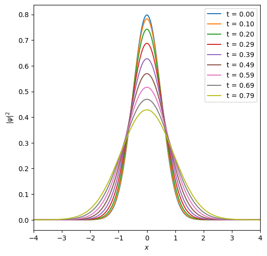
Exercise 2: Plot the evolution of the probability distribution

Let’s plot the evolution of the probability distribution every 2 time steps (i.e. \(2\epsilon = T_0/64\)) from \(t=0\) to \(T_0/8 = \pi/4\).

plt.figure(figsize=(6, 6))
plot_interval = 2
for i in range(0, NT // 8 + 1, plot_interval):
    # plot the probability distribution and label it with the time
    plt.plot(x, prob[i], label=f"t = {t[i]:.2f}")
plt.xlabel(r"$x$")
plt.ylabel(r"$|\psi|^2$")
plt.xlim([xmin, xmax])
plt.legend()
plt.show()

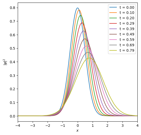
Changing the initial wave function

It seems like the mean position of the particle doesn’t move, but the probability does “disperse” away. Why is that? The initial wave function is a Gaussian centered at \(x_\mathrm{start} = 0\) basically representing a particle at rest. But this has contributions from all possible momenta, so the particle has some probability to be found away from the origin with amplitude given according to the free propagator.

Let’s try a different wave function with some definite initial momentum \(p=\hbar k_0\),

\[\Psi_0(x) = \left(\frac{\alpha}{\pi}\right)^{1/4}\exp\left(-\frac{\alpha}{2}(x-x_\mathrm{start})^2 + i k_0 (x-x_\mathrm{start})\right),\]

and again \(\alpha = 2\) and \(x_\mathrm{start} = 0\), and now let’s set the wavenumber \(k_0 = 1\) .

K0 = 1

def func_psi_0(x, x_start):
    alpha = 2
    return (alpha / np.pi) ** (1 / 4) * np.exp(-(alpha / 2) * (x - x_start)**2 + 1j * K0 * (x - x_start))

psi_0 = func_psi_0(x, XSTART)

print(f"Psi at every 10th point: {psi_0[::10]}")
print(f"Normalization condition:  {DELTAX * sum(psi_0 * psi_0.conjugate())}")

Psi at every 10th point: [-6.57051404e-08+7.60748099e-08j -2.14757315e-07+1.90293299e-07j
 -6.56043983e-07+4.40913794e-07j -1.88446904e-06+9.29922775e-07j
 -5.10920025e-06+1.72195465e-06j -1.31051826e-05+2.54405021e-06j
 -3.18458859e-05+1.86215170e-06j -7.33586815e-05-5.50678032e-06j
 -1.60184435e-04-3.38507128e-05j -3.31325369e-04-1.17796053e-04j
 -6.48208888e-04-3.33295093e-04j -1.19651826e-03-8.33172789e-04j
 -2.07555022e-03-1.90123366e-03j -3.36167620e-03-4.02473830e-03j
 -5.02859711e-03-7.97570457e-03j -6.80830026e-03-1.48764075e-02j
 -7.98806465e-03-2.62060846e-02j -7.16464603e-03-4.36912322e-02j
 -2.01628493e-03-6.90225398e-02j  1.08029825e-02-1.03370247e-01j
  3.55138407e-02-1.46733565e-01j  7.66873157e-02-1.97251404e-01j
  1.38301698e-01-2.50693343e-01j  2.22476424e-01-3.00397059e-01j
  3.28149355e-01-3.37875229e-01j  4.50101551e-01-3.54159205e-01j
  5.78761491e-01-3.41702783e-01j  7.01086016e-01-2.96414413e-01j
  8.02525291e-01-2.19228065e-01j  8.69715784e-01-1.16654209e-01j
  8.93243842e-01+0.00000000e+00j  8.69715784e-01+1.16654209e-01j
  8.02525291e-01+2.19228065e-01j  7.01086016e-01+2.96414413e-01j
  5.78761491e-01+3.41702783e-01j  4.50101551e-01+3.54159205e-01j
  3.28149355e-01+3.37875229e-01j  2.22476424e-01+3.00397059e-01j
  1.38301698e-01+2.50693343e-01j  7.66873157e-02+1.97251404e-01j
  3.55138407e-02+1.46733565e-01j  1.08029825e-02+1.03370247e-01j
 -2.01628493e-03+6.90225398e-02j -7.16464603e-03+4.36912322e-02j
 -7.98806465e-03+2.62060846e-02j -6.80830026e-03+1.48764075e-02j
 -5.02859711e-03+7.97570457e-03j -3.36167620e-03+4.02473830e-03j
 -2.07555022e-03+1.90123366e-03j -1.19651826e-03+8.33172789e-04j
 -6.48208888e-04+3.33295093e-04j -3.31325369e-04+1.17796053e-04j
 -1.60184435e-04+3.38507128e-05j -7.33586815e-05+5.50678032e-06j
 -3.18458859e-05-1.86215170e-06j -1.31051826e-05-2.54405021e-06j
 -5.10920025e-06-1.72195465e-06j -1.88446904e-06-9.29922775e-07j
 -6.56043983e-07-4.40913794e-07j -2.14757315e-07-1.90293299e-07j
 -6.57051404e-08-7.60748099e-08j]
Normalization condition:  (0.999999999999998+2.1223432016435976e-19j)

psi = [psi_0]

for i in range(1, NT + 1):
    psi_t = DELTAX * np.matmul(K_dt, psi[i-1])
    psi.append(psi_t)

prob = []
for i in range(NT + 1):
    prob.append(np.real(psi[i] * psi[i].conjugate()))

Exercise 3: Plot the evolution of the probability distribution

Again, let’s plot the evolution of the probability distribution every 2 time steps (i.e. \(2\epsilon = T_0/64\)) from \(t=0\) to \(T_0/8 = \pi/4\).

plt.figure(figsize=(6, 6))
for i in range(0, NT // 8 + 1, plot_interval):
    # plot the probability distribution and label it with the time
    plt.plot(x, prob[i], label=f"t = {t[i]:.2f}")
plt.xlabel(r"$x$")
plt.ylabel(r"$|\psi|^2$")
plt.xlim([xmin, xmax])
plt.legend()
plt.show()